Deep Learning for Anomaly Detection
FF12 · ©2020 Cloudera, Inc. All rights reserved


This is an applied research report by Cloudera Fast Forward Labs. We write reports about emerging technologies. Accompanying each report are working prototypes that exhibit the capabilities of the algorithm and offer detailed technical advice on its practical application. Read our full report on using deep learning for anomaly detection below or download the PDF. For this report we built two prototypes: Blip and Anomagram.
Introduction
“An outlier is an observation which deviates so much from other observations as to arouse suspicions that it was generated by a different mechanism.”
– Hawkins, Identification of Outliers (1980)
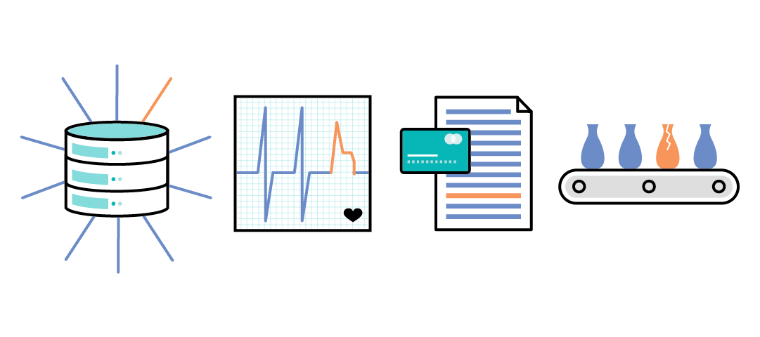
Anomalies, often referred to as outliers, abnormalities, rare events, or deviants, are data points or patterns in data that do not conform to a notion of normal behavior. Anomaly detection, then, is the task of finding those patterns in data that do not adhere to expected norms, given previous observations. The capability to recognize or detect anomalous behavior can provide highly useful insights across industries. Flagging unusual cases or enacting a planned response when they occur can save businesses time, costs, and customers. Hence, anomaly detection has found diverse applications in a variety of domains, including IT analytics, network intrusion analytics, medical diagnostics, financial fraud protection, manufacturing quality control, marketing and social media analytics, and more.
Applications of Anomaly Detection
We’ll begin by taking a closer look at some possible use cases, before diving into different approaches to anomaly detection in the next chapter.
Network Intrusion Detection
Network security is critical to running a modern viable business, yet all computer systems suffer from security vulnerabilities which are both technically difficult and economically punishing to resolve once exploited. Business IT systems collect data about their own network traffic, user activity in the system, types of connection requests, and more. While most activity will be benign and routine, analysis of this data may provide insights into unusual (anomalous) activity within the network after and ideally before a substantive attack. In practice, the damage and cost incurred right after an intrusion event escalates faster than most teams are able to mount an effective response. Thus, it becomes critical to have special-purpose intrusion detection systems (IDSs) in place that can surface potential threat events and anomalous probing early and in a reliable manner.
Medical Diagnosis
In many medical diagnosis applications, a variety of data points (e.g., X-rays, MRIs, ECGs) indicative of health status are collected as part of diagnostic processes. Some of these data points are also collected by end-user medical devices (e.g., glucose monitors, pacemakers, smart watches). Anomaly detection approaches can be applied to highlight situations of abnormal readings that may be indicative of health conditions or precursor signals of medical incidents.
Fraud Detection
In 2018, fraud was estimated to have a global financial cost of over £3.89 trillion (about $5 trillion USD). Within the financial services industry, it is critical for service providers to quickly and correctly identify and react to fraudulent transactions. In the most straightforward cases, a transaction may be identified as fraudulent by comparison to the historical transactions by a given party or to all other transactions occurring within the same time period for a peer group. Here, fraud can be cast as a deviation from normal transaction data and addressed using anomaly detection approaches. Even as financial fraud is further clustered into card-based, check-based, unauthorized account access-based, or authorized payment-based categories, the core concepts of baselining an individual’s standard behavior and looking for signals of unusual activity apply.
Manufacturing Defect Detection
Within the manufacturing industry, an automated approach to the task of detecting defects, particularly in items manufactured in large volumes, is vital to quality assurance (QA). This task can be cast as an anomaly detection exercise, where the goal is to identify manufactured items that significantly or even slightly differ from ideal (normal) items that have passed QA tests. The amount of acceptable deviation is determined by the company and customers, as well as industry and regulatory standards.
Use-Case Example
ScoleMans has been making drywall panels for years and is the leading regional supplier for construction companies. Occasionally, some of the wall panels they produce have defects: cracks, chips at the edges, paint/coating issues, etc. As part of their QA process, they capture both RGB and thermal images of each produced panel, which their QA engineers use to flag defective units. They want to automate this process; i.e., develop tools that automatically identify these defects. This is possible using a deep anomaly detection model. In particular, ScoleMans can use an autoencoder or GAN-based model built with convolutional neural network blocks (see Chapter 3. Deep Learning for Anomaly Detection for more information) to create a model of normal data based on images of normal panels. This model can then be used to tag new images as normal or abnormal.
Similarly, the task of predictive maintenance can be cast as an anomaly detection problem. For example, anomaly detection approaches can be applied to data from machine sensors (vibrations, temperature, drift, and more), where abnormal sensor readings can be indicative of impending failures.
As these examples suggest, anomaly detection is useful in a variety of areas. Detecting and correctly classifying as anomalous something previously unseen is a challenging problem that has been tackled in many different ways over the years. While there are many approaches, the traditional machine learning (ML) techniques are suboptimal when it comes to high-dimensional data and sequence datasets, because they fail to capture the complex structures in the data.
This report, with its accompanying prototype, explores deep learning-based approaches that first learn to model normal behavior and then exploit this knowledge to identify anomalies. While they’re capable of yielding remarkable results on complex and high-dimensional data, there are several factors that influence the choice of approach when building an anomaly detection application. We survey the options, highlighting their pros and cons.
Background
In this chapter, we provide an overview of approaches to anomaly detection based on the type of data available, how to evaluate an anomaly detection model, how each approach constructs a model of normal behavior, and why deep learning models are valuable. We conclude with a discussion of pitfalls that may be encountered while deploying these models.
Anomaly Detection Approaches
Anomaly detection approaches can be categorized in terms of the type of data needed to train the model. In most use cases, it is expected that anomalous samples represent a very small percentage of the entire dataset. Thus, even when labeled data is available, normal data samples are more readily available than abnormal samples. This assumption is critical for most applications today. In the following sections, we touch on how the availability of labeled data impacts the choice of approach.
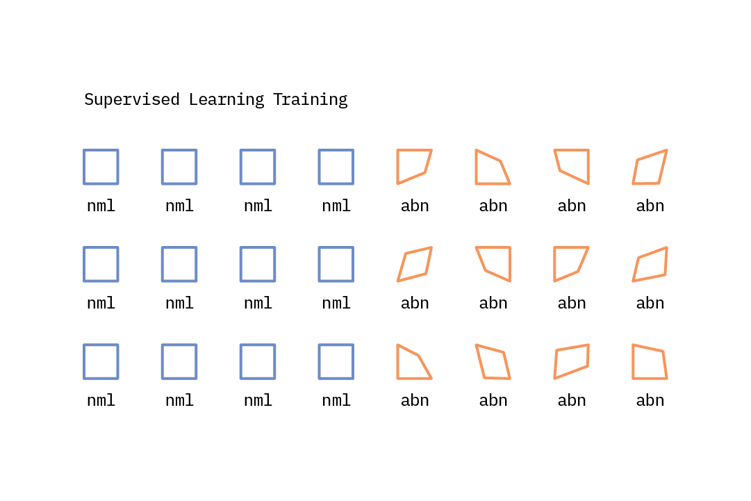
Supervised Learning
When learning with supervision, machines learn a function that maps input features to outputs based on example input-output pairs. The goal of supervised anomaly detection algorithms is to incorporate application-specific knowledge into the anomaly detection process. With sufficient normal and anomalous examples, the anomaly detection task can be reframed as a classification task where the machines can learn to accurately predict whether a given example is an anomaly or not. That said, for many anomaly detection use cases the proportion of normal versus anomalous examples is highly imbalanced; while there may be multiple anomalous classes, each of them could be quite underrepresented.
This approach assumes that one has labeled examples for all types of anomalies that could occur and can correctly classify them. In practice, this is usually not the case, as anomalies can take many different forms, with novel anomalies emerging at test time. Thus, approaches that generalize well and are more effective at identifying previously unseen anomalies are preferable.
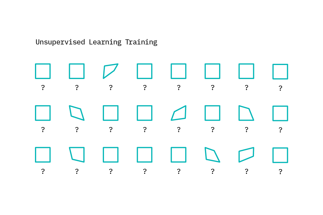
Unsupervised learning
With unsupervised learning, machines do not possess example input-output pairs that allow it to learn a function that maps the input features to outputs. Instead, they learn by finding structure within the input features. Because, as mentioned previously, labeled anomalous data is relatively rare, unsupervised approaches are more popular than supervised ones in the anomaly detection field. That said, the nature of the anomalies one hopes to detect is often highly specific. Thus, many of the anomalies found in a completely unsupervised manner could correspond to noise, and may not be of interest for the task at hand.
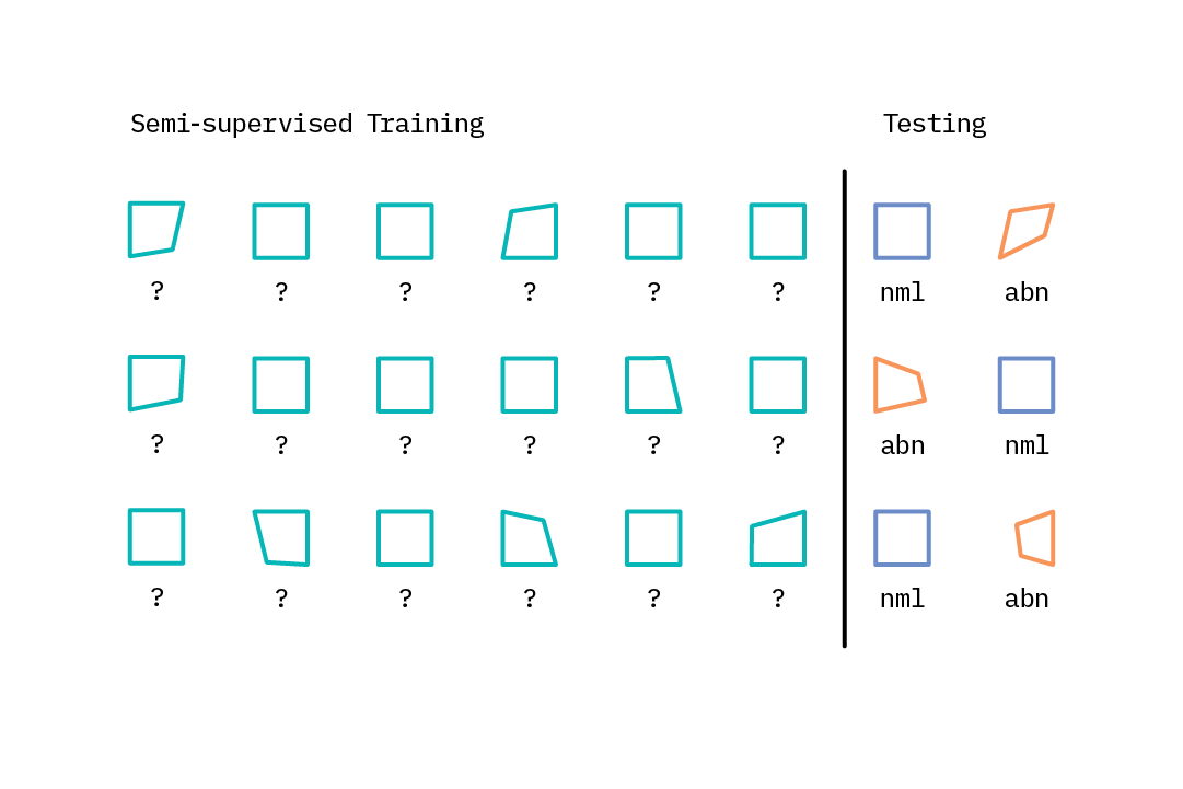
Semi-supervised learning
Semi-supervised learning approaches represent a sort of middle ground, employing a set of methods that take advantage of large amounts of unlabeled data as well as small amounts of labeled data. Many real-world anomaly detection use cases are well suited to semi-supervised learning, in that there are a huge number of normal examples available from which to learn, but relatively few examples of the more unusual or abnormal classes of interest. Following the assumption that most data points within an unlabeled dataset are normal, one can train a robust model on an unlabeled dataset and evaluate its performance (and tune the model’s parameters) using a small amount of labeled data.[1]
This hybrid approach is well suited to applications like network intrusion detection, where one may have multiple examples of the normal class and some examples of intrusion classes, but new kinds of intrusions may arise over time.
To give another example, consider X-ray screening for aviation or border security. Anomalous items posing a security threat are not commonly encountered and can take many forms. In addition, the nature of any anomaly posing a potential threat may evolve due to a range of external factors. Exemplary data of anomalies can therefore be difficult to obtain in any useful quantity.
Such situations may require the determination of abnormal classes as well as novel classes, for which little or no labeled data is available. In cases like these, a semi-supervised classification approach that enables detection of both known and previously unseen anomalies is an ideal solution.
Evaluating Models: Accuracy Is Not Enough
As mentioned in the previous section, in anomaly detection applications it is expected that the distribution between the normal and abnormal class(es) may be highly skewed. This is commonly referred to as the class imbalance problem. A model that learns from such skewed data may not be robust; it may be accurate when classifying examples within the normal class, but perform poorly when classifying anomalous examples.
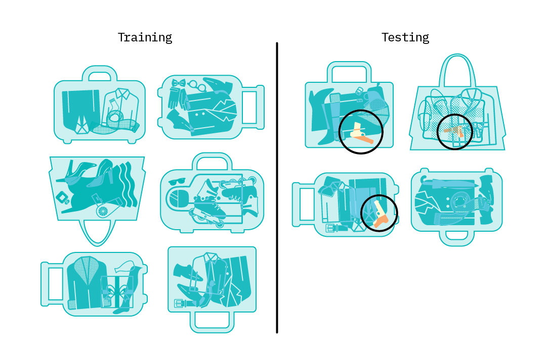
For example, consider a dataset consisting of 1,000 images of luggage passing through a security checkpoint. 950 images are of normal pieces of luggage, and 50 are abnormal. A classification model that always classifies an image as normal can achieve high overall accuracy for this dataset (95%), even though its accuracy rate for classifying abnormal data is 0%.
Such a model may also misclassify normal examples as anomalous (false positives, FP), or misclassify anomalous examples as normal ones (false negatives, FN). As we consider both of these types of errors, it becomes obvious that the traditional accuracy metric (total number of correct classifications divided by total classifications) is insufficient in evaluating the skill of an anomaly detection model.
Two important metrics have been introduced that provide a better measure of model skill: precision and recall. Precision is defined as the number of true positives (TP) divided by the number of true positives plus the number of false positives (FP), while recall is the number of true positives divided by the number of true positives plus the number of false negatives (FN). Depending on the use case or application, it may be desirable to optimize for either precision or recall.
Optimizing for precision may be useful when the cost of failure is low, or to reduce human workload. Optimizing for high recall may be more appropriate when the cost of a false negative is very high; for example, in airport security, where it is better to flag many items for human inspection (low cost) in order to avoid the much higher cost of incorrectly admitting a dangerous item onto a flight. While there are several ways to optimize for precision or recall, the manner in which a threshold is set can be used to reflect the precision and recall preferences for each specific use case.
You now have an idea of why an unsupervised or semi-supervised approach to anomaly detection is desirable, and what metrics are best to use for evaluating these models. In the next section, we focus on semi-supervised approaches and discuss how they work.
Anomaly Detection as Learning Normal Behavior
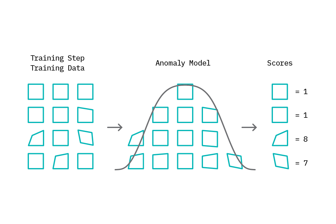
The underlying strategy for most approaches to anomaly detection is to first model normal behavior, and then exploit this knowledge to identify deviations (anomalies). This approach typically falls under the semi-supervised learning category and is accomplished through two steps in the anomaly detection loop. The first step, referred to as the training step, involves building a model of normal behavior using available data. Depending on the specific anomaly detection method, this training data may contain both normal and abnormal data points, or only normal data points (see Chapter 3. Deep Learning for Anomaly Detection for additional details on anomaly detection methods). Based on this model, an anomaly score is then assigned to each data point that represents a measure of deviation from normal behavior.
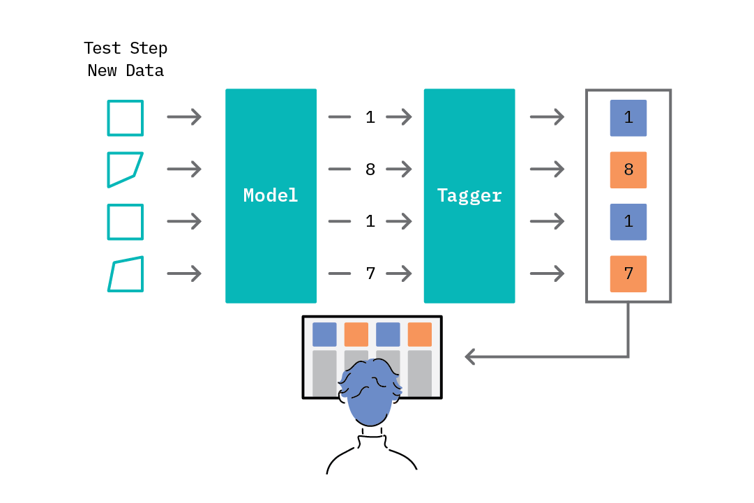
The second step in the anomaly detection loop, the test step, introduces the concept of threshold-based anomaly tagging. Based on the range of scores assigned by the model, one can select a threshold rule that drives the anomaly tagging process; e.g., scores above a given threshold are tagged as anomalies, while those below it are tagged as normal. The idea of a threshold is valuable, as it provides the analyst an easy lever with which to tune the “sensitivity” of the anomaly tagging process. Interestingly, while most methods for anomaly detection follow this general approach, they differ in how they model normal behavior and generate anomaly scores.
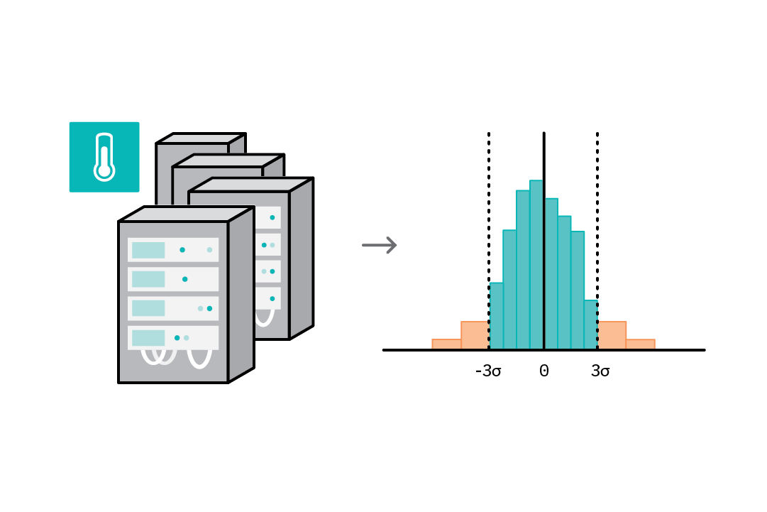
To further illustrate this process, consider the scenario where the task is to detect abnormal temperatures (e.g., spikes), given data from the temperature sensors attached to servers in a data center. We can use a statistical approach to solve this problem (see the table in the following section for an overview of common methods). In step 1, we assume the samples follow a normal distribution, and we can use sample data to learn the parameters of this distribution (mean and variance). We assign an anomaly score based on a sample’s deviation from the mean and set a threshold (e.g., any value more than 3 standard deviations from the mean is an anomaly). In step 2, we then tag all new temperature readings and generate a report.
Approaches to Modeling Normal Behavior
Given the importance of the anomaly detection task, multiple approaches haveR been proposed and rigorously studied over the last few decades. To provide a high-level summary, we categorize the more popular techniques into four main areas: clustering, nearest neighbor, classification, and statistical. For a detailed survey of existing techniques, see [2]). The following table provides a summary of the assumptions and anomaly scoring strategies employed by approaches within each category, and some examples of each.
| Anomaly Detection Method | Assumptions | Anomaly Scoring | Notable Examples |
|---|---|---|---|
| Clustering | Normal data points belong to a cluster (or lie close to its centroid) in the data while anomalies do not belong to any clusters. | Distance from nearest cluster centroid | Self-organizing maps (SOMs), k-means clustering, expectation maximization (EM) |
| Nearest Neighbour | Normal data instances occur in dense neighborhoods while anomalous data are far from their nearest neighbors | Distance from _k_th nearest neighbour | k-nearest neighbors (KNN) |
| Classification |
|
A measure of classifier estimate (likelihood) that a data point belongs to the normal class | One-class support vector machines (OCSVMs) |
| Statistical | Given an assumed stochastic model, normal data instances fall in high-probability regions of the model while abnormal data points lie in low-probability regions | Probability that a data point lies in a high-probability region in the assumed distribution | Regression models (ARMA, ARIMA) |
| Deep learning | Given an assumed stochastic model, normal data instances fall in high-probability regions of the model while abnormal data points lie in low-probability regions | Probability that a data point lies in a high-probability region in the assumed distribution | autoencoders, sequence-to-sequence models, generative adversarial networks (GANs), variational autoencoders (VAEs) |
The majority of these approaches have been applied to univariate time series data; a single data point generated by the same process at various time steps (e.g., readings from a temperature sensor over time); and assume linear relationships within the data. Examples include k-means clustering, ARMA, ARIMA, etc. However, data is increasingly high-dimensional (e.g., multivariate datasets, images, videos), and the detection of anomalies may require the joint modeling of interactions between each variable. For these sorts of problems, deep learning approaches (the focus of this report) such as autoencoders, VAEs, sequence-to-sequence models, and GANs present some benefits.
Why Use Deep Learning for Anomaly Detection?
Deep learning approaches, when applied to anomaly detection, offer several advantages. First, these approaches are designed to work with multivariate and high dimensional data. This makes it easy to integrate information from multiple sources, and eliminates challenges associated with individually modeling anomalies for each variable and aggregating the results. Deep learning approaches are also well-adapted to jointly modeling the interactions between multiple variables with respect to a given task and - beyond the specification of generic hyperparameters (number of layers, units per layer, etc.) - deep learning models require minimal tuning to achieve good results.
Performance is another advantage. Deep learning methods offer the opportunity to model complex, nonlinear relationships within data, and leverage this for the anomaly detection task. The performance of deep learning models can also potentially scale with the availability of appropriate training data, making them suitable for data-rich problems.
What Can Go Wrong?
There are a proliferation of algorithmic approaches that can help one tackle an anomaly detection task and build solid models, at times even with just normal samples. But do they really work? What could possibly go wrong? Here are some of the issues that need to be considered:
Contaminated normal examples
In large-scale applications that have huge volumes of data, it’s possible
that within the large unlabeled dataset that’s considered the normal class,
a small percentage of the examples may actually be anomalous, or simply be poor training
examples. And while some models (like a one-class SVM or isolation forest) can
account for this, there are others that may not be robust to detecting
anomalies.
Computational complexity
Anomaly detection scenarios can sometimes have low latency requirements; i.e., it may be necessary to be able to speedily retrain existing models as new data becomes available, and
perform inference. This can be computationally expensive at scale, even for
linear models for univariate data. Deep learning models also incur
additional compute costs to estimate their large number of parameters. To
address these issues, it is recommended to explore trade-offs that
balance the frequency of retraining and overall accuracy.
Human supervision
One major challenge with unsupervised and semi-supervised approaches is that
they can be noisy and may generate a large amount of false positives. In turn,
false positives incur labor costs associated with human review. Given these
costs, an important goal for anomaly detection systems is to incorporate the
results of human review (as labels) to improve model quality.
Definition of anomaly
In many data domains, the boundary between normal and anomalous behavior is not precisely
defined and is continually evolving. Unlike in other task
domains where dataset shift occurs sparingly, anomaly detection systems
should anticipate and account for (frequent) changes in the distribution of the
data. In many cases, this can be achieved by frequent retraining of the models.
Threshold selection
The process of selecting a good threshold value can be challenging. In a
semi-supervised setting (the approaches covered above), one has access to a pool
of labeled data. Using these labels, and some domain expertise, it is possible to
determine a suitable threshold. Specifically, one can explore the range of
anomaly scores for each data point in the validation set and select as a threshold
the point that yields the best performance metric (accuracy, precision,
recall). In the absence of labeled data, and assuming that most data points
are normal, one can use statistics such as standard deviation and percentiles to
infer a good threshold.
Interpretability
Deep learning methods for anomaly detection can be complex, leading to their reputation as black
box models. However, interpretability techniques such as LIME (see our previous report,
“Interpretability”) and Deep SHAP provide opportunities for analysts to inspect
their behavior and make them more interpretable.
Deep Learning for Anomaly Detection
In this chapter, we will review a set of relevant deep learning model architectures and how they can be applied to the task of anomaly detection. As discussed in Chapter 2. Background, anomaly detection involves first teaching a model to recognize normal behavior, then generating anomaly scores that can be used to identify anomalous activity.
The deep learning approaches discussed here typically fall within a family of encoder-decoder models: an encoder that learns to generate an internal representation of the input data, and a decoder that attempts to reconstruct the original input based on this internal representation. While the exact techniques for encoding and decoding vary across models, the overall benefit they offer is the ability to learn the distribution of normal input data and construct a measure of anomaly respectively.
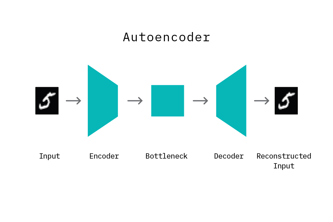
Autoencoders
Autoencoders are neural networks designed to learn a low-dimensional representation, given some input data. They consist of two components: an encoder that learns to map input data to a low-dimensional representation (termed the bottleneck), and a decoder that learns to map this low-dimensional representation back to the original input data. By structuring the learning problem in this manner, the encoder network learns an efficient “compression” function that maps input data to a salient lower-dimensional representation, such that the decoder network is able to successfully reconstruct the original input data. The model is trained by minimizing the reconstruction error, which is the difference (mean squared error) between the original input and the reconstructed output produced by the decoder. In practice, autoencoders have been applied as a dimensionality reduction technique, as well as in other use cases such as noise removal from images, image colorization, unsupervised feature extraction, and data compression.
It is important to note that the mapping function learned by an autoencoder is specific to the training data distribution. That is, an autoencoder will typically not succeed at reconstructing data that is significantly different from the data it has seen during training. As we will see later in this chapter, this property of learning a distribution-specific mapping (as opposed to a generic linear mapping) is particularly useful for the task of anomaly detection.
Modeling Normal Behavior and Anomaly Scoring
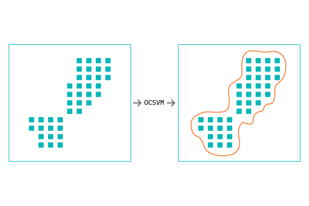
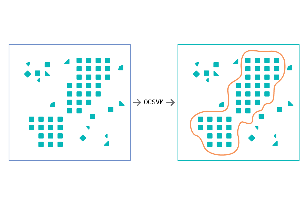
Applying an autoencoder for anomaly detection follows the general principle of first modeling normal behavior and subsequently generating an anomaly score for each new data sample. To model normal behavior, we follow a semi-supervised approach where we train the autoencoder on normal data samples. This way, the model learns a mapping function that successfully reconstructs normal data samples with a very small reconstruction error. This behavior is replicated at test time, where the reconstruction error is small for normal data samples, and large for abnormal data samples. To identify anomalies, we use the reconstruction error score as an anomaly score and flag samples with reconstruction errors above a given threshold.
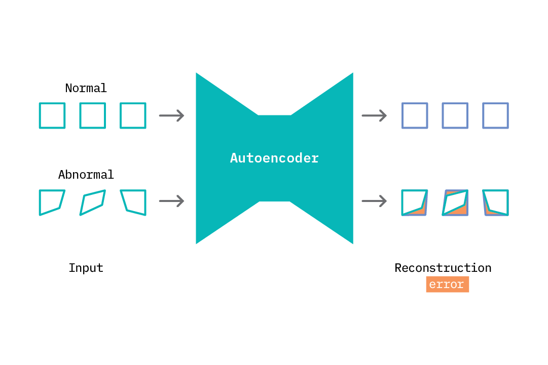
This process is illustrated in the figure above. As the autoencoder attempts to reconstruct abnormal data, it does so in a manner that is weighted toward normal samples (square shapes). The difference between what it reconstructs and the input is the reconstruction error. We can specify a threshold and flag anomalies as samples with a reconstruction error above a given threshold.
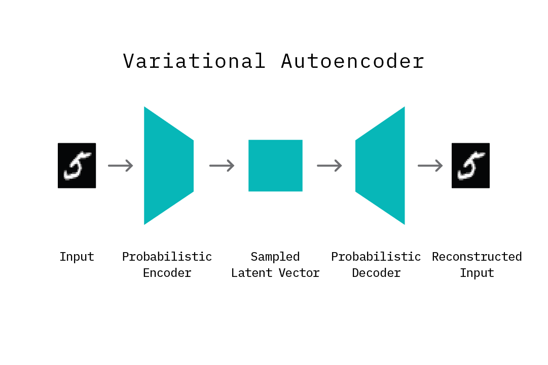
Variational Autoencoders
A variational autoencoder (VAE) is an extension of the autoencoder. Similar to an autoencoder, it consists of an encoder and a decoder network component, but it also includes important changes in the structure of the learning problem to accommodate variational inference. As opposed to learning a mapping from the input data to a fixed bottleneck vector (a point estimate), a VAE learns a mapping from an input to a distribution, and learns to reconstruct the original data by sampling from this distribution using a latent code. In Bayesian terms, the prior is the distribution of the latent code, the likelihood is the distribution of the input given the latent code, and the posterior is the distribution of the latent code, given our input. The components of a VAE serve to derive good estimates for these terms.
The encoder network learns the parameters (mean and variance) of a distribution that outputs a latent code vector Z, given the input data (posterior). In other words, one can draw samples of the bottleneck vector that “correspond” to samples from the input data. The nature of this distribution can vary depending on the nature of the input data (e.g., while Gaussian distributions are commonly used, Bernoulli distributions can be used if the input data is known to be binary). On the other hand, the decoder learns a distribution that outputs the original input data point (or something really close to it), given a latent bottleneck sample (likelihood). Typically, an isotropic Gaussian distribution is used to model this reconstruction space.
The VAE model is trained by minimizing the difference between the estimated distribution produced by the model and the real distribution of the data. This difference is estimated using the Kullback-Leibler divergence, which quantifies the distance between two distributions by measuring how much information is lost when one distribution is used to represent the other. Similar to autoencoders, VAEs have been applied in use cases such as unsupervised feature extraction, dimensionality reduction, image colorization, image denoising, etc. In addition, given that they use model distributions, they can be leveraged for controlled sample generation.
The probabilistic Bayesian components introduced in VAEs lead to a few useful benefits. First, VAEs enable Bayesian inference; essentially, we can now sample from the learned encoder distribution and decode samples that do not explicitly exist in the original dataset, but belong to the same data distribution. Second, VAEs learn a disentangled representation of a data distribution; i.e., a single unit in the latent code is only sensitive to a single generative factor. This allows some interpretability of the output of VAEs, as we can vary units in the latent code for controlled generation of samples. Third, a VAE provides true probability measures that offer a principled approach to quantifying uncertainty when applied in practice (for example, the probability that a new data point belongs to the distribution of normal data is 80%).
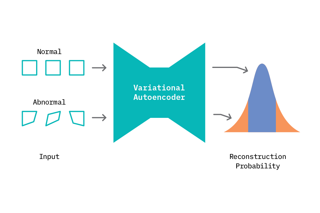
Modeling Normal Behavior and Anomaly Scoring
Similar to an autoencoder, we begin by training the VAE on normal data samples. At test time, we can compute an anomaly score in two ways. First, we can draw samples of the latent code Z from the encoder given our input data, sample reconstructed values from the decoder using Z, and compute a mean reconstruction error. Anomalies are flagged based on some threshold on the reconstruction error.
Alternatively, we can output a mean and a variance parameter from the decoder, and compute the probability that the new data point belongs to the distribution of normal data on which the model was trained. If the data point lies in a low-density region (below some threshold), we flag that as an anomaly. We can do this because we’re modeling a distribution as opposed to a point estimate.
Generative Adversarial Networks
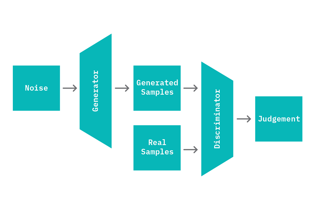
Generative adversarial networks (GANs[3]) are neural networks designed to learn a generative model of an input data distribution. In their classic formulation, they’re composed of a pair of (typically feed-forward) neural networks termed a generator, G, and discriminator, D. Both networks are trained jointly and play a competitive skill game with the end goal of learning the distribution of the input data, X.
The generator network G learns a mapping from random noise of a fixed dimension (Z) to samples X_ that closely resemble members of the input data distribution. The discriminator D learns to correctly discern real samples that originated in the source data (X) from fake samples (X_) that are generated by G. At each epoch during training, the parameters of G are updated to maximize its ability to generate samples that are indistinguishable by D, while the parameters of D are updated to maximize its ability to to correctly discern true samples X from generated samples X_. As training progresses, G becomes proficient at producing samples that are similar to X, and D also upskills on the task of distinguishing real from fake samples.
In this classic formulation of GANs, while G learns to model the source distribution X well (it learns to map random noise from Z to the source distribution), there is no straightforward approach that allows us to harness this knowledge for controlled inference; i.e., to generate a sample that is similar to a given known sample. While we can conduct a broad search over the latent space with the goal of recovering the most representative latent noise vector for an arbitrary sample, this process is compute-intensive and very slow in practice.
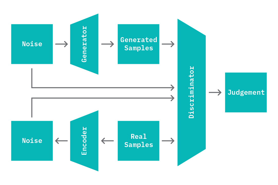
To address these issues, recent research studies have explored new formulations of GANs that enable just this sort of controlled adversarial inference by introducing an encoder network, E (BiGANs[4]) with applications in anomaly detection (See GANomaly[5][6]). In simple terms, the encoder learns the reverse mapping of the generator; it learns to generate a fixed vector Z_, given a sample. Given this change, the input to the discriminator is also modified; the discriminator now takes in pairs of input that include the latent representation (Z, and Z_), in addition to the data samples (X and X_). The encoder E is then jointly trained with the generator G; G learns an induced distribution that outputs samples of X given a latent code Z, while E learns an induced distribution that outputs Z, given a sample X.
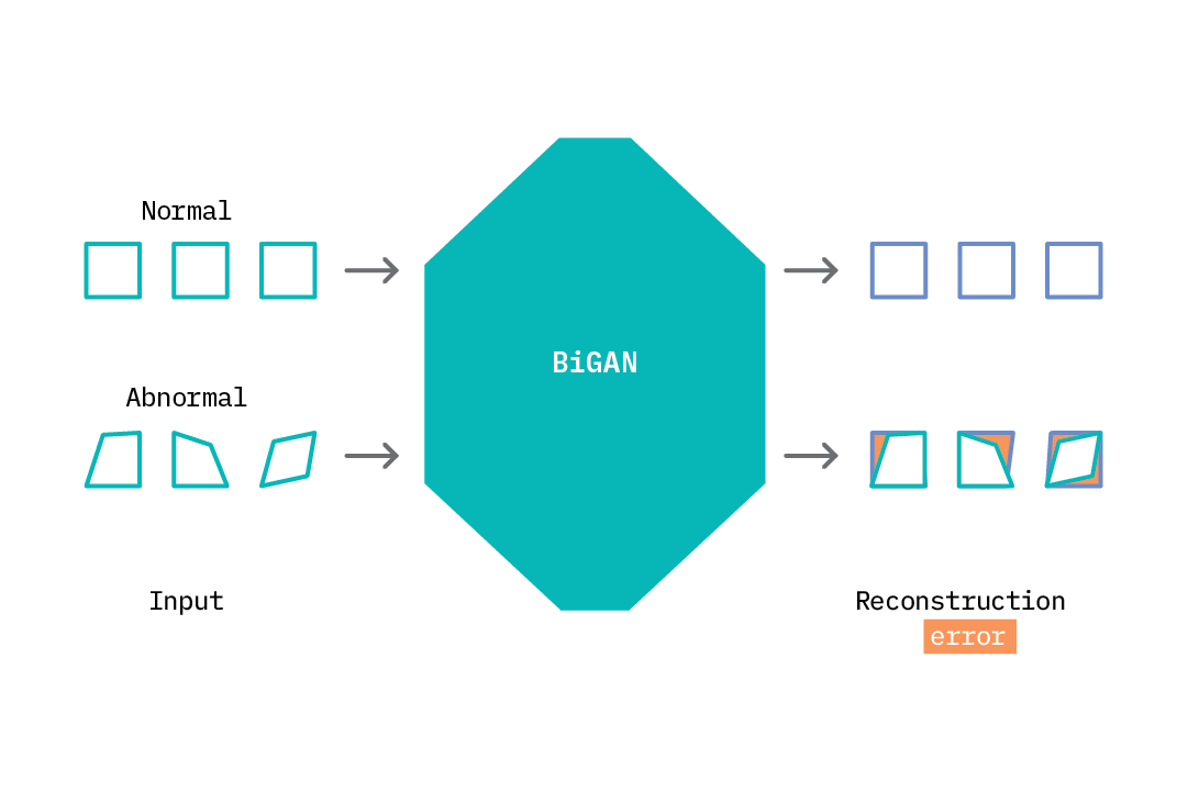
Again, the mappings learned by components in the GAN are specific to the data used in training. For example, the generator component of a GAN trained on images of cars will always output an image that looks like a car, given any latent code. At test time, we can leverage this property to infer how different a given input sample is from the data distribution on which the model was trained.
Modeling Normal Behavior and Anomaly Scoring
To model normal behavior, we train a BiGAN on normal data samples. At the end of the training process, we have an encoder E that has learned a mapping from data samples (X) to latent code space (Z_), a discriminator D that has learned to distinguish real from generated data, and a generator G that has learned a mapping from latent code space to sample space. Note that these mappings are specific to the distribution of normal data that has been seen during training. At test time, we perform the following steps to generate an anomaly score for a given sample X. First, we obtain a latent space value Z_ from the encoder given X, which is fed to the generator and yields a sample X_. Next, we can compute an anomaly score based on the reconstruction loss (difference between X and X_) and the discriminator loss (cross entropy loss or feature differences in the last dense layer of the discriminator, given both X and X_).
Sequence-to-Sequence Models
Sequence-to-sequence models are a class of neural networks mainly designed to learn mappings between data that are best represented as sequences. Data containing sequences can be challenging as each token in a sequence may have some form of temporal dependence on other tokens; a relationship that has to be modeled to achieve good results. For example, consider the task of language translation where a sequence of words in one language needs to be mapped to a sequence of words in a different language. To excel at such a task, a model must take into consideration the (contextual) location of each word/token within the broader sentence; this allows it to generate an appropriate translation (See our previous report on Natural Language Processing to learn more about this area.)
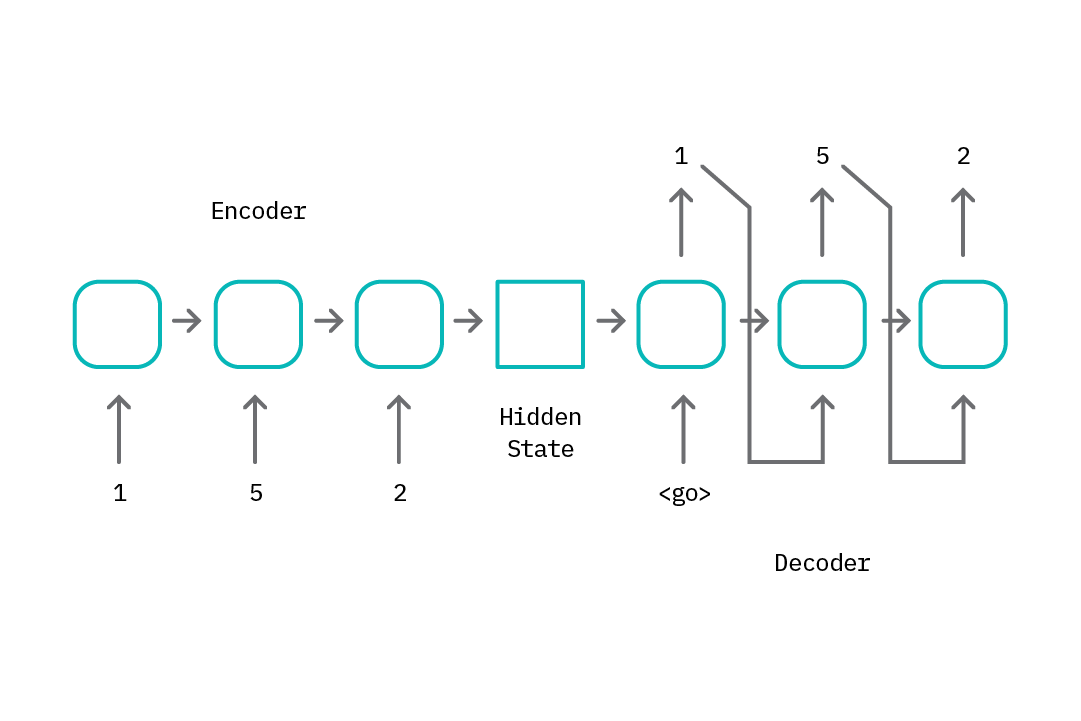
On a high level, sequence-to-sequence models typically consist of an encoder, E, that generates a hidden representation of the input tokens, and a decoder, D, that takes in the encoder representation and sequentially generates a set of output tokens. Traditionally, the encoder and decoder are composed of long short-term memory (LSTM) blocks, that are particularly suitable for modeling temporal relationships within input data tokens.
While sequence-to-sequence models excel at modeling data with temporal dependence, they can be slow during inference; each individual token in the model output is sequentially generated at each time step, where the total number of steps is the length of the output token.
We can use this encoder-decoder structure for anomaly detection by revising the sequence-to-sequence model to function like an autoencoder, training the model to output the same tokens as the input, shifted by 1. This way, the encoder learns to generate a hidden representation that allows the decoder to reconstruct input data that is similar to examples seen in the training dataset.
Modeling Normal Behavior and Anomaly Scoring
To identify anomalies, we take a semi-supervised approach where we train the sequence-to-sequence model on normal data. At test time, we can then compare the difference (mean squared error) between the output sequence generated by the model and its input. As in the approaches discussed previously, we can use this value as an anomaly score.
One-Class Support Vector Machines
In this section, we discuss one-class support vector machines (OCSVMs), a non-deep learning approach to classification that we will use later (see Chapter 4. Prototype) as a baseline.
Traditionally, the goal of classification approaches is to help distinguish between different classes, using some training data. However, consider a scenario where we have data for only one class, and the goal is to determine whether test data samples are similar to the training samples. OCSVMs were introduced for exactly this sort of task: novelty detection, or the detection of unfamiliar samples. SVMs have proven very popular for classification, and they introduced the use of kernel functions to create nonlinear decision boundaries (hyperplanes) by projecting data into a higher dimension. Similarly, OCSVMs learn a decision function which specifies regions in the input data space where the probability density of the data is high. An OCSVM model is trained with various hyperparameters:
nuspecifies the fraction of outliers (data samples that do not belong to our class of interest) that we expect in our data.kernelspecifies the kernel type to be used in the algorithm; examples include RBF, polynomial (poly), and linear. This enables SVMs to use a nonlinear function to project the input data to a higher dimension.gammais a parameter of the RBF kernel type that controls the influence of individual training samples; this affects the “smoothness” of the model.
Modeling Normal Behavior and Anomaly Scoring
To apply OCSVM for anomaly detection, we train an OCSVM model using normal data, or data containing a small fraction of abnormal samples. Within most implementations of OCSVM, the model returns an estimate of how similar a data point is to the data samples seen during training. This estimate may be the distance from the decision boundary (the separating hyperplane), or a discrete class value (+1 for data that is similar and -1 for data that is not). Either type of score can be used as an anomaly score.
Additional Considerations
In practice, applying deep learning relies on a few data and modeling assumptions. This section explores them in detail.
Anomalies as Rare Events
For the training approaches discussed thus far, we operate on the assumption of the availability of “normal” labeled data, which is then used to teach a model recognize normal behavior. In practice, it is often the case that labels do not exist or can be expensive to obtain. However, it is also a common observation that anomalies (by definition) are relatively infrequent events and therefore constitute a small percentage of the entire event dataset (for example, the occurrence of fraud, machine failure, cyberattacks, etc.). Our experiments (see Chapter 4. Prototype for more discussion) have shown that the neural network approaches discussed above remain robust in the presence of a small percentage of anomalies (less than 10%). This is mainly because introducing a small fraction of anomalies does not significantly affect the network’s model of normal behavior. For scenarios where anomalies are known to occur sparingly, our experiments show that it’s possible to relax the requirement of assembling a dataset consisting only of labeled normal samples for training.
Discretizing Data and Handling Stationarity
To apply deep learning approaches for anomaly detection (as with any other task), we need to construct a dataset of training samples. For problem spaces where data is already discrete, we can use the data as is (e.g., a dataset of images of wall panels, where the task is to find images containing abnormal panels). When data exists as a time series, we can construct our dataset by discretizing the series into training samples. Typically this involves slicing the data into chunks with comparable statistical properties. For example, given a series of recordings generated by a data center temperature sensor, we can discretize the data into daily or weekly time slices and construct a dataset based on these chunks. This becomes our basis for anomaly comparison (e.g., the temperature pattern for today is anomalous compared to patterns for the last 20 days). The choice of the discretization approach (daily, weekly, averages, etc.) will often require some domain expertise; the one requirement is that each discrete sample be comparable. For example, given that temperatures may spike during work hours compared to non-work hours in the scenario we’re considering, it may be challenging to discretize this data by hour as different hours exhibit different statistical properties.
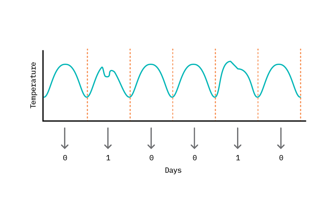
This notion of constructing a dataset of comparable samples is related to the idea of stationarity. A stationary series is one in which properties of the data (mean, variance) do not vary with time. Examples of non-stationary data include data containing trends (e.g., rising global temperatures) or with seasonality (e.g., hourly temperatures within each day). These variations need to be handled during discretization. We can remove trends by applying a differencing function to the entire dataset. To handle seasonality, we can explicitly include information on seasonality as a feature of each discrete sample; for instance, to discretize by hour, we can attach a categorical variable representing the hour of the day. A common misconception regarding the application of neural networks capable of modeling temporal relationships such as LSTMs is that they automatically learn/model properties of the data useful for predictions (including trends and seasonality). However, the extent to which this is possible is dependent on how much of this behavior is represented in each training sample. For example, to automatically account for trends or patterns across the day, we can discretize data by hour with an additional categorical feature for hour of day, or discretize by day (24 features for each hour).
Note: For most machine learning algorithms, it is a requirement that samples be independent and identically distributed. Ensuring we construct comparable samples (i.e., handle trends and seasonality) from time series data allows us to satisfy the latter requirement, but not the former. This can affect model performance. In addition, constructing a dataset in this way raises the possibility that the learned model may perform poorly in predicting output values that lie outside the distribution (range of values) seen during training; i.e., if there is a distribution shift. This greatly amplifies the need to retrain the model as new data arrives, and complicates the model deployment process. In general, discretization should be applied with care.
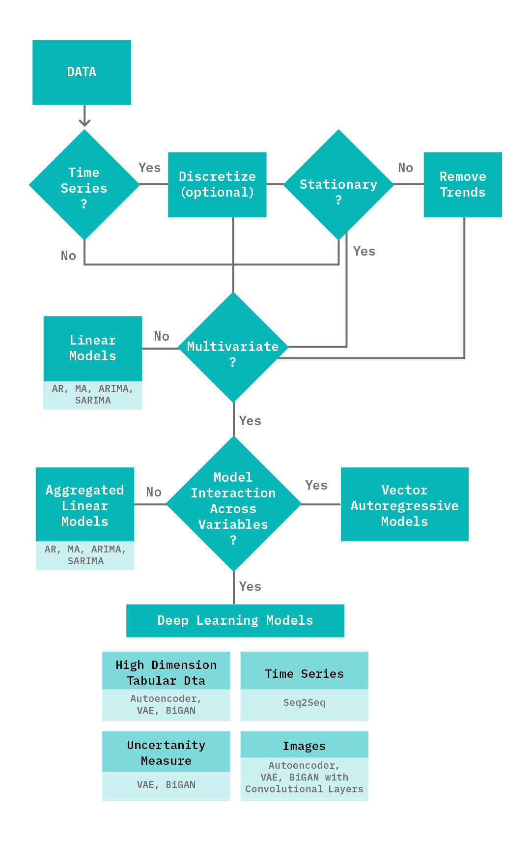
Selecting a Model
There are several factors that can influence the primary approach taken when it comes to detecting anomalies. These include the data properties (time series vs. non-time series, stationary vs. non-stationary, univariate vs. multivariate, low-dimensional vs. high-dimensional), latency requirements, uncertainty reporting, and accuracy requirements. More importantly, deep learning methods are not always the best approach! To provide a framework for navigating this space, we offer the following recommendations:
Data Properties
-
Time series data: As discussed in the previous section, it is important to correctly discretize the data and to handle stationarity before training a model. In addition, for discretized data with temporal relationships, the use of LSTM layers as part of the encoder or decoder can help model these relationships.
-
Univariate vs Multivariate: Deep learning methods are well suited to data that has a wide range of features: they’re recommended for high-dimensional data, such as images, and work well for modeling the interactions between multiple variables. For most univariate datasets, linear models (see Chandola et al.) are both fast and accurate and thus typically preferred.
Business Requirements
-
Latency: Deep learning models are slower than linear models. For scenarios that include high volumes of data and have low latency requirements, linear models are recommended (e.g., for detecting anomalies in authentication requests for 200,000 work sites, with each machine generating 500 requests per second).
-
Accuracy: Deep learning approaches tend to be robust, providing better accuracy, precision, and recall.
-
Uncertainty: For scenarios where it is a requirement to provide a principled estimate of uncertainty for each anomaly classification, deep learning models such as VAEs and BiGANs are recommended.
How to Decide on a Modeling Approach?
Given the differences between the deep learning methods discussed above (and their variants), it can be challenging to decide on the right model. When data contains sequences with temporal dependencies, a sequence-to-sequence model (or architectures with LSTM layers) can model these relationships, yielding better results. For scenarios requiring principled estimates of uncertainty, generative models such as a VAE and GAN based approaches are suitable. For scenarios where the data is images, AEs, VAEs and GANs designed with convolution layers are suitable.
The following table highlights the pros and cons of the different types of models, to give you an idea under what kind of scenarios they are recommended.
| Model | Pros | Cons |
|---|---|---|
| AutoEncoder |
|
|
| Variational AutoEncoder |
|
|
| GAN (BiGAN) |
|
|
| Sequence-to-Sequence Model |
|
|
| One Class SVM |
|
|
Prototype
In this section, we provide an overview of the data and experiments used to evaluate each of the approaches mentioned in Chapter 3. Deep Learning for Anomaly Detection. We also introduce two prototypes we built to demonstrate results from the experiments and how we designed each prototype.
Datasets
KDD
The KDD network intrusion dataset is a dataset of TCP connections that have been labeled as normal or representative of network attacks.
“A connection is a sequence of TCP packets starting and ending at some well-defined times, between which data flows to and from a source IP address to a target IP address under some well-defined protocol.”
These attacks fall into four main categories - denial of service, unauthorized access from a remote machine, unauthorized access to local superuser privileges, and surveillance, e.g., port scanning. Each TCP connection is represented as a set of attributes or features (derived based on domain knowledge) pertaining to each connection such as the number of failed logins, connection duration, data bytes from source to destination, etc. The dataset is comprised of a training set (97278 normal traffic samples, 396743 attack traffic samples) and a test set (63458 normal packet samples, 185366 attack traffic samples). To make the data more realistic, the test portion of the dataset contains 14 additional attack types that are not in the train portion; thus, a good model should generalize well and detect attacks unseen during training.
ECG5000
The ECG5000 dataset contains examples of ECG signals from a patient. Each data sample, which corresponds to an extracted heartbeat containing 140 points, has been labeled as normal or being indicative of heart conditions related to congestive heart failure. Given an ECG signal sample, the task is to predict if it is normal or abnormal. ECG5000 is well-suited to a prototype for a few reasons: it is visual (signals can be visualized easily) and it is based on real data associated with a concrete use case (heart disease detection). While the task itself is not extremely complex, the data is multivariate (140 values per sample, which allows us to demonstrate the value of a deep model), but small enough to rapidly train and run inference.
Benchmarking Models
We sought to compare each of the models discussed earlier using the KDD dataset. We preprocessed the data to keep only 18 continuous features (Note: this slightly simplifies the problem and results in differences from similar benchmarks on the same dataset). Feature scaling (0-1 minmax scaling) is also applied to the data; scaling parameters are learned from training data and then applied to test data. We then trained each model using normal samples (97,278 samples) and evaluated it on a random subset of the test data (8000 normal samples and 2000 normal samples).
| Method | Encoder | Decoder | Other Parameters |
|---|---|---|---|
| PCA | NA | NA | 2 Component PCA |
| OCSVM | NA | NA | Kernel: Rbf, Outlier fraction: 0.01; gamma: 0.5. Anomaly score as distance from decision boundary. |
| Autoencoder | 2 hidden layers [15, 7] | 2 hidden layers [15, 7] | Latent dimension: 2Batch size: 256Loss: Mean squared error |
| Variational Autoencoder | 2 hidden layers [15, 7] | 2 hidden layers [15, 7] | Latent dimension: 2 Batch size: 256 Loss: Mean squared error + KL divergence |
| Sequence to Sequence Model | 1 hidden layer, [10] | 1 hidden layer [20] | Bidirectional LSTMs Batch size: 256 Loss: Mean squared error |
| Bidirectional GAN | Encoder: 2 hidden layers [15, 7], Generator: 2 hidden layers [15, 7] |
Generator: 2 hidden layers [15, 7] Discriminator: 2 hidden layers [15, 7] | Latent dimension: 32 Loss: Binary Cross Entropy Learning rate: 0.1 |
We implemented each model using comparable parameters (see the table above) that allow us to benchmark them in terms of training and inference (total training time to best accuracy, inference time), storage (size of weights, number of parameters), and performance (accuracy, precision, recall). The deep learning models (AE, VAE, Seq2seq, BiGAN) were implemented in Tensorflow (keras api); each model was trained till best accuracy measured on the same validation dataset, using the Adam optimizer, batch size of 256 and a learning rate of 0.01. OCSVM was implemented using the Sklearn OCSVM library using the non-linear rbf kernel and parameters (nu=0.01 and gamma=0.5). Results from PCA (using the the sum of the projected distance of a sample on all eigenvectors as the anomaly score) are also included. Additional details on the parameters for each model are summarized in the table below for reproducibility. These experiments were run on an Intel® Xeon® CPU @ 2.30GHz and a NVIDIA T4 GPU (applicable to the deep models).
Training, Inference, Storage
| Method | Model Size (KB) | Inference Time (Seconds) | # of Parameters | Total Training Time (Seconds) |
|---|---|---|---|---|
| BiGAN | 47.945 | 1.26 | 714 | 111.726 |
| Autoencoder | 22.008 | 0.279 | 842 | 32.751 |
| OCSVM | 10.77 | 0.029 | NA | 0.417 |
| VAE | 23.797 | 0.391 | 858 | 27.922 |
| Seq2Seq | 33.109 | 400.131 | 2741 | 645.448 |
| PCA | 1.233 | 0.003 | NA | 0.213 |
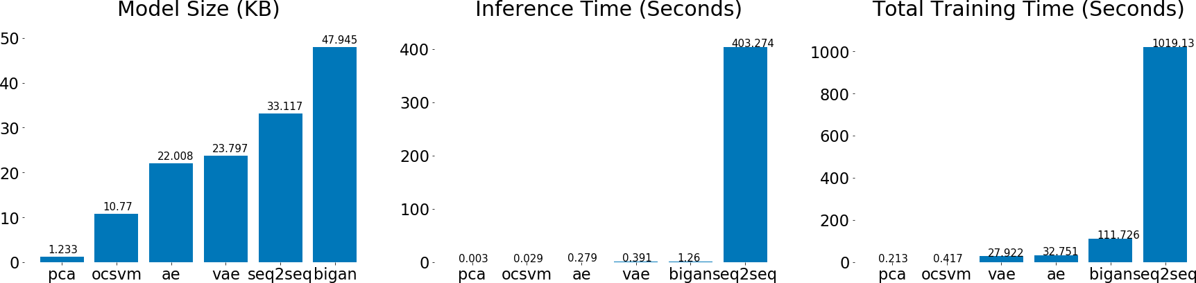
Each model is compared in terms of inference time on the entire test dataset, total training time to peak accuracy, number of parameters (deep models), and model size.
As expected, a linear model like PCA is both fast to train and fast for inference. This is followed by OCSVM, autoencoders, variational autoencoders, BiGAN, and sequence-to-sequence models in order of increasing model complexity. The GAN-based model required the most training epochs to achieve stable results; this is in part due to a known stability issue associated with GANs. The sequence-to-sequence model is particularly slow for inference given the sequential nature of the decoder.
For each of the deep models, we store the network weights to disk and compute the size of weights. For OCSVM and PCA, we serialize the model to disk using pickle and compute the size of each model file. These values are helpful in estimating memory and storage costs when deploying these models in production.
Performance
| Method | ROC AUC | Accuracy | Precision | Recall | F1 score | F2 Score |
|---|---|---|---|---|---|---|
| BiGAN | 0.972 | 0.962 | 0.857 | 0.973 | 0.911 | 0.947 |
| Autoencoder | 0.963 | 0.964 | 0.867 | 0.968 | 0.914 | 0.945 |
| OCSVM | 0.957 | 0.949 | 0.906 | 0.83 | 0.866 | 0.844 |
| VAE | 0.946 | 0.93 | 0.819 | 0.836 | 0.827 | 0.832 |
| Seq2Seq | 0.919 | 0.829 | 0.68 | 0.271 | 0.388 | 0.308 |
| PCA | 0.771 | 0.936 | 0.977 | 0.699 | 0.815 | 0.741 |
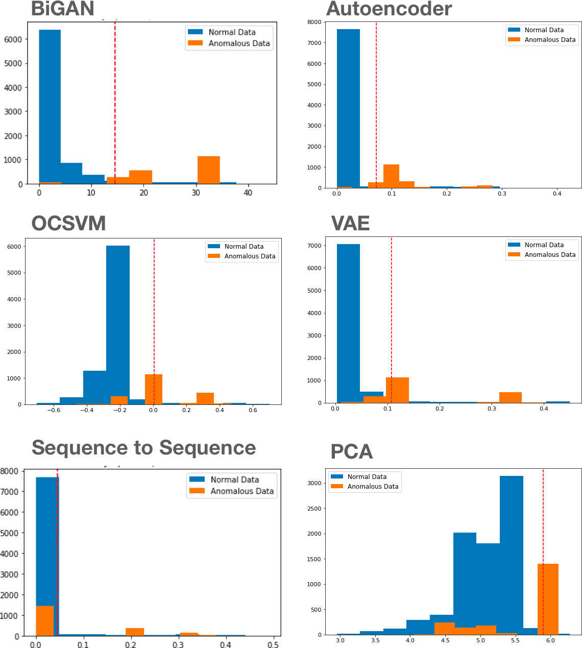
For each model, we use labeled test data to first select a threshold that yields the best accuracy and then report on metrics such as f1, f2, precision, and recall at that threshold. We also report on ROC (area under the curve) to evaluate the overall skill of each model. Given that the dataset we use is not extremely complex (18 features), we see that most models perform relatively well. Deep models (BiGAN, AE) are more robust (precision, recall, ROC AUC), compared to PCA and OCSVM. The sequence-to-sequence model is not particularly competitive, given the data is not temporal. On a more complex dataset (e.g., images), we expect to see (similar to existing research), more pronounced advantages in using a deep learning model.
Web Application Prototypes
We built two prototypes that demonstrate results and insights from our experiments. The first prototype, Blip, is built on on the KDD dataset used in the experiments above and is a visualization of the performance of four approaches to anomaly detection. The second prototype, Anomagram, is an interactive explainer that focuses on the autoencoder model, and the results from applying it to detecting anomalies in ECG data.
Blip
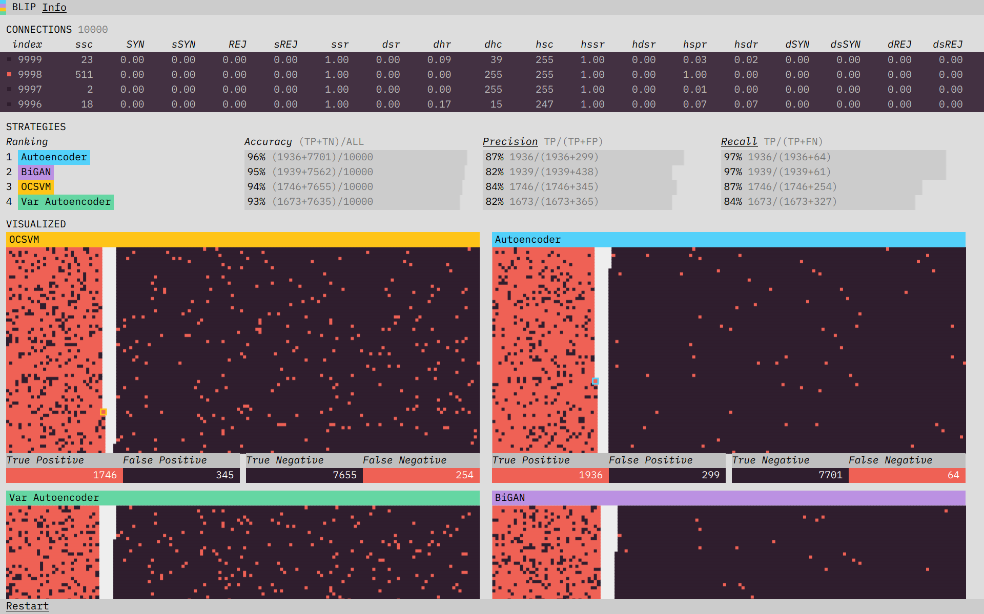
Blip plays back and visualizes the performance of four different algorithms on a subset of the KDD network intrusion dataset. Blip dramatizes the analogy detection process and builds user intution about the trade-offs involved.
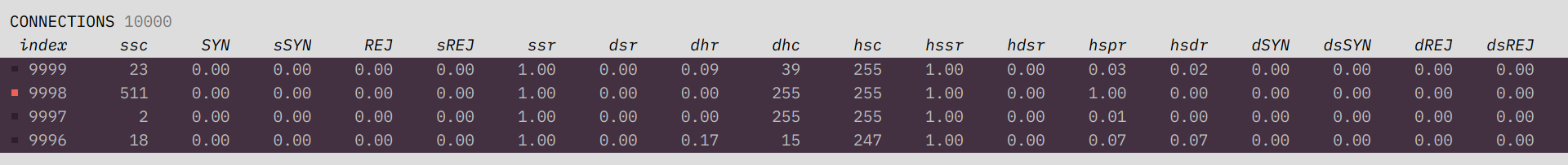
The concept of an anomaly is easy to visualize: something that doesn’t look the same. The conceptual simplicity of it actually makes the prototype’s job tricker. If we show you a dataset where the anomalies are easy to spot, it’s not clear what you need an algorithm for. Instead, we want to place you in a situation where the data is complicated enough, and streaming in fast enough, that the benefits of an algorithm are clear. Often in a data visualization, you want to remove complexity; in Blip, we wanted to preserve it, but place it in context. We did this by including at the top a terminal-like view of the connection data coming in. The speed and number of features involved make the usefulness of an algorithm, which can operate at a higher speed and scale than a human, clear.

Directly below the terminal-like streaming data, we show performance metrics for each of the algorithms. These metrics include accuracy, recall, and precision. The three different measurements hint at the trade-offs involved in choosing an anomaly detection algorithm. You will want to prioritize different metrics depending on the situation. Accuracy is a measure of how often the algorithm is right. Prioritizing precision will minimize false positives, while focusing on recall will minimize false negatives. By showing the formulas for each of these metrics, updated in real-time with the streaming data, we build intuition about how the different measures interact.
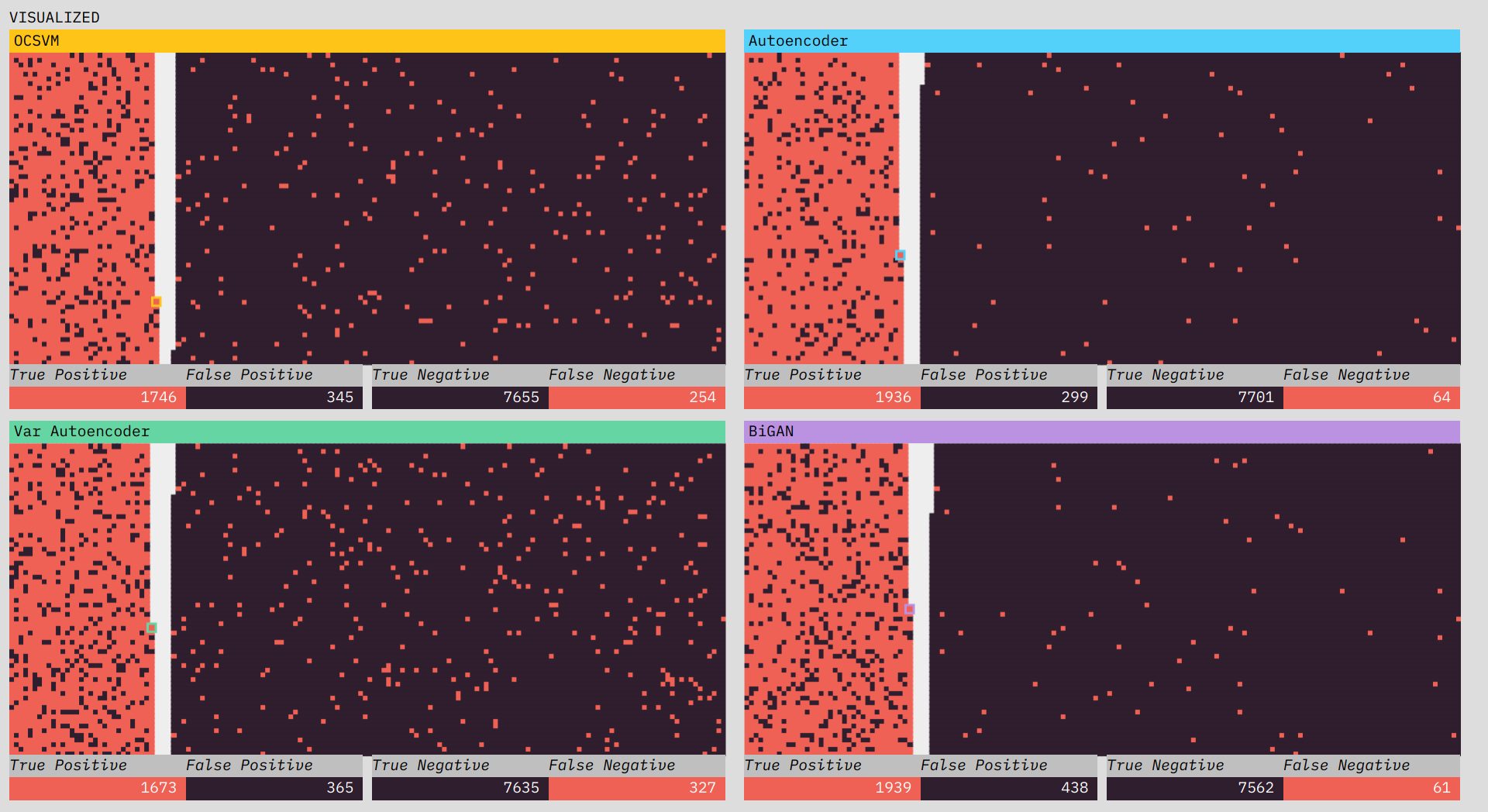
In the visualizations, we want to give the user a feel for how each algorithm performs across the various metrics. If a connection is classified by the algorithm as an anomaly, it is stacked on the left; if it is classified as normal, it is placed on the right. The ground truth is indicated by the color: red for anomaly, black for normal. In a perfectly performing algorithm, the left side would be completely red and the right completely black. An algorithm that has lots of false negatives (low recall) will have a higher density of red mixed in with the black on the right side. A low precision performance will show up as lots of black mixed into the left side. The fact that each connection gets its own spot makes the scale of the dataset clear (versus the streaming-terminal view where old connections quickly leave the screen). Our ability to quickly assess visual density makes it easier to get a feel for what differences in performance metrics across algorithms really mean.
One difficulty in designing the prototype was figuring out when to reveal the ground truth (visualized as the red or black color). In a real-world situation, you would not know the truth as it came in (you woudn’t need an algorithm then). Early versions of the prototype experimented with only revealing the color after classification. Ultimately, we decided that because there is already a lot happening in the prototype, a delayed reveal pushed the complexity a step too far. Part of this is because the prototype shows the performance of four different algorithms. If we were showing only one, we’d have more room to animate the truth reveal. We decided to reveal the color truth at the start to strengthen the visual connection between the connection data as shown in the terminal and in each of the algorithm visualizations.
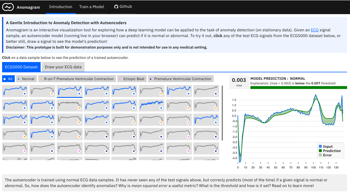
Prototype II - Anomagram
This section describes Anomagram - an interactive web based experience where the user can build, train and evaluate an autoencoder to detect anomalous ECG signals. It utilizes the ECG5000 dataset mentioned above.
UX Goals for Anomagram
Anomagram is designed as part of a growing area of interactive visualizations (see Neural Network Playground, ConvNet Playground, GANLab, GAN dissection, etc.) that help communicate technical insights on how deep learning models work. It is entirely browser-based and implemented in Tensorflow.js. This way, users can explore live experiments with no installations required. Importantly, Anomagram moves beyond the use of toy/synthetic data and situates learning within the context of a concrete task (anomaly detection for ECG data). The overall user experience goals for Anomagram are summarized as follows:
1: Provide an introduction to autoencoders and how they can be applied to the task of anomaly detection. This is achieved via the Introduction module (see screenshot below). This entails providing definitions of concepts (reconstruction error, thresholds, etc.) paired with interactive visualizations that demonstrate concepts (e.g., an interactive visualization for inference on test data, a visualization of the structure of an autoencoder, a visualization of error histograms as training progresses, etc.).
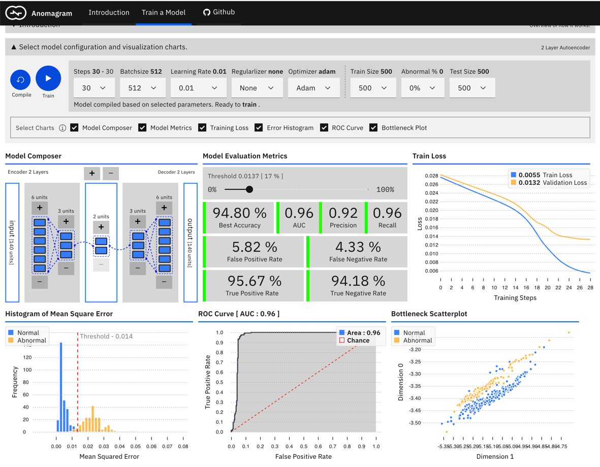
2: Provide an interactive, accessible experience that supports technical learning by doing. This is mostly accomplished within the Train a Model module (see screenshot below) and is designed for users interested in additional technical depth. It entails providing a direct manipulation interface that allows the user to specify a model (add/remove layers and units within layers), modify model parameters (training steps, batchsize, learning rate, regularizer, optimizer), modify training/test data parameters (data size, data composition), train the model, and evaluate model performance (visualization of accuracy, precision, recall, false positive, false negative, ROC, etc. metrics) as each parameter is changed. Who should use Anomagram? Anyone interested to learn about autoencoders and anomaly detection in an accessible way. Anomagram is also useful for educators (as a tool to support guided discussion of the topic), entry level data scientists, and non-ML experts (citizen data scientists, software developers, designers).
Interface Affordances and Insights
This section discusses some explorations the user can perform with Anomagram, and some corresponding insights.
Craft (Adversarial) Input: Anomalies by definition can take many different and previously unseen forms. This makes the assessment of anomaly detection models more challenging. Ideally, we want the user to conduct their own evaluations of a trained model, e.g., by allowing them to upload their own ECG data. In practice, this requires the collection of digitized ECG data with similar preprocessing (heartbeat extraction) and range as the ECG5000 dataset used in training the model. This is challenging. The next best way to allow testing on examples contributed by the user is to provide a simulator — hence the draw your ECG data feature. This provides an (html) canvas on which the user can draw signals and observe the model’s behaviour. Drawing strokes are converted to an array, with interpolation for incomplete drawings (total array size=140) and fed to the model. While this approach has limited realism (users may not have sufficient domain expertise to draw meaningful signals), it provides an opportunity to craft various types of (adversarial) samples and observe the model’s performance.
Insights: The model tends to expect reconstructions that are close to the mean of normal data samples. Using the Draw your ECG data feature, the user can draw (adversarial) examples of input data and observe model predictions/performance.
Visually Compose a Model: Users can intuitively specify an autoencoder architecture using a direct manipulation model composer. They can add layers and add units to layers using clicks. The architecture is then used to specify the model’s parameters each time the model is compiled. This follows a similar approach used in “A Neural Network Playground”[3]. The model composer connector lines are implemented using the leaderline library. Relevant lines are redrawn or added as layers are added or removed from the model.
Insights: There is no marked difference between a smaller model (1 layer) and a larger model (e.g., 8 layers) for the current task. This is likely because the task is not especially complex (a visualization of PCA points for the ECG dataset suggests it is linearly separable). Users can visually compose the autoencoder model — add remove layers in the encoder and decoder. To keep the encoder and decoder symmetrical, add/remove operations on either are mirrored.
Effect of Learning Rate, Batchsize, Optimizer, Regularization: The user can select from 6 optimizers (Adam, Adamax, Adadelta, Rmsprop, Momentum, Sgd), various learning rates, and regularizers (l1, l2, l1l2).
Insights: Adam reaches peak accuracy with less steps compared to other optimizers. Training time increases with no benefit to accuracy as batchsize is reduced (when using Adam). A two layer model will quickly overfit on the data; adding regularization helps address this to some extent.
Effect of Threshold Choices on Precision/Recall: Earlier in this report (see Chapter 2. Evaluating Models: Accuracy Is Not Enough ) we highlight the importance of metrics such as precision and recall and why accuracy is not enough. To support this discussion, the user can visualize how threshold choices impact each of these metrics.
Insights: As threshold changes, accuracy can stay the same but, precision and recall can vary. This further illustrates how the threshold can be used by an analyst as a lever to reflect their precision/recall preferences.
Effect of Data Composition: We may not always have labeled normal data to train a model. However, given the rarity of anomalies (and domain expertise), we can assume that unlabeled data is mostly comprised of normal samples. However, this assumption raises an important question - does model performance degrade with changes in the percentage of abnormal samples in the dataset? In the Train a Model section, you can specify the percentage of abnormal samples to include when training the autoencoder model.
Insights: We see that with 0% abnormal data, the model AUC is ~96%. Great! At 30% abnormal sample composition, AUC drops to ~93%. At 50% abnormal data points, there is just not enough information in the data that allows the model to learn a pattern of normal behaviour. It essentially learns to reconstruct normal and abnormal data well and mse is no longer a good measure of anomaly. At this point, model performance is only slightly above random chance (AUC of 56%).
Landscape
This chapter provides an overview of the landscape of currently available open source tools and service vendor offerings available for anomaly detection, and considers the trade-offs as well as when to use each.
Open Source Tools and Frameworks
Several popular open source machine learning libraries and packages in Python and R
include implementations of algorithmic techniques that can be applied to anomaly
detection tasks. Useful algorithms (e.g., clustering, OCSVMs, isolation forests) also exist
as part of general-purpose frameworks like scikit-learn that do not cater
specifically to anomaly detection. In addition, generic packages for univariate
time series forecasting (e.g., Facebook’s
Prophet) have been applied widely to
anomaly detection tasks where anomalies are identified based on the difference
between the true value and a forecast.
In this section, our focus is on comprehensive toolboxes that specifically address the task of anomaly detection.
Python Outlier Detection (PyOD)
PyOD is an open source Python toolbox for performing scalable outlier detection on multivariate data. It provides access to a wide range of outlier detection algorithms, including established outlier ensembles and more recent neural network-based approaches, under a single, well-documented API.
PyOD offers several distinct advantages:
- It gives access to over 20 algorithms, ranging from classical techniques such as local outlier factor (LOF) to recent neural network architectures such as autoencoders and adversarial models.
- It implements combination methods for merging the results of multiple detectors and outlier ensembles, which are an emerging set of models.
- It includes a unified API, detailed documentation, and interactive examples across all algorithms for clarity and ease of use.
- All models are covered by unit testing with cross-platform continuous integration, code coverage, and code maintainability checks.
- Optimization instruments are employed when possible: just-in-time (JIT) compilation and parallelization are enabled in select models for scalable outlier detection.
- It’s compatible with both Python 2 and 3 across major operating systems.
Seldon’s Anomaly Detection Package
Seldon.io is known for its open source ML deployment solution for
Kubernetes, which can in principle be used to serve arbitrary models. In
addition, the Seldon team has recently released
alibi-detect, a Python package
focused on outlier, adversarial, and concept drift detection. The package aims
to provide both online and offline detectors for tabular data, text, images, and
time series data. The outlier detection methods should allow the user to identify
global, contextual, and collective outliers.
Seldon has identified anomaly detection as a sufficiently important capability to warrant dedicated attention in the framework, and has implemented several models to use out of the box. The existing models include sequence-to-sequence LSTMs, variational autoencoders, spectral residual models for time series, Gaussian mixture models, isolation forests, Mahalanobis distance, and others. Examples and documentation are provided.
In the Seldon Core architecture, anomaly detection methods may be implemented as either models or input transformers. In the latter case, they can be composed with other data transformations to process inputs to another model. This nicely illustrates one role anomaly detection can play in ML systems: flagging bad inputs before they pass through the rest of a pipeline.
R Packages
The following section reviews R packages that have been created for anomaly detection. Interestingly, most of them deal with time series data.
Twitter’s AnomalyDetection package
Twitter’s AnomalyDetection is an open source R package that can be used to automatically detect anomalies. It is applicable across a wide variety of contexts (for example, anomaly detection in system metrics after a new software release, user engagement after an A/B test, or problems in econometrics, financial engineering, or the political and social sciences). It can help detect both global and local anomalies as well as positive/negative anomalies (i.e., a point-in-time increase/decrease in values).
The primary algorithm, Seasonal Hybrid Extreme Studentized Deviate (S-H-ESD), builds upon the Generalized ESD test for detecting anomalies, which can be either global or local. This is achieved by employing time series decomposition and using robust statistical metrics; i.e., median together with ESD. In addition, for long time series (say, 6 months of minutely data), the algorithm employs piecewise approximation.
The package can also be used to detect anomalies in a vector of numerical values when the corresponding timestamps are not available, and it provides rich visualization support. The user can specify the direction of anomalies and the window of interest (such as the last day or last hour) and enable or disable piecewise approximation, and the x- and y-axes are annotated to assist visual data analysis.
anomalize package
The anomalize package, open sourced by Business Science, performs time series anomaly detection that goes inline with other Tidyverse
packages (or packages
supporting tidy data).
Anomalize has three main functions:
- Decompose separates out the time series into seasonal, trend, and remainder components.
- Anomalize applies anomaly detection methods to the remainder component.
- Recompose calculates upper and lower limits that separate the “normal” data from the anomalies.
tsoutliers package
This package implements a procedure based on the approach described in Chen and Liu (1993) for automatic detection of outliers in time series. Time series data often undergoes nonsystematic changes that alter the dynamics of the data, either transitorily or permanently. The approach considers innovational outliers, additive outliers, level shifts, temporary changes, and seasonal level shifts while fitting a time series model.
Numenta’s HTM (Hierarchical Temporal Memory)
Research organization Numenta has introduced a machine intelligence framework for anomaly detection called Hierarchical Temporal Memory (HTM). At the core of HTM are time-based learning algorithms that store and recall temporal patterns. Unlike most other ML methods, HTM algorithms learn time-based patterns in unlabeled data on a continuous basis. They are robust to noise and high-capacity, meaning they can learn multiple patterns simultaneously. The HTM algorithms are documented and available through the open source Numenta Platform for Intelligent Computing (NuPIC). They’re particularly suited to problems involving streaming data and to identifying underlying patterns in data change over time, subtle patterns, and time-based patterns.
One of the first commercial applications to be developed using NuPIC is Grok, a tool that performs IT analytics, giving insight into IT systems to identify unusual behavior and reduce business downtime. Another is Cortical.io, which enables applications in natural language processing.
The NuPIC platform also offers several tools, such as HTM Studio and Numenta Anomaly Benchmark (NAB). HTM Studio is a free desktop tool that enables developers to find anomalies in time series data without the need to program, code, or set parameters. NAB is a novel benchmark for evaluating and comparing algorithms for anomaly detection in streaming, real-time applications. It is composed of over 50 labeled real-world and artificial time series data files, plus a novel scoring mechanism designed for real-time applications.
Besides this, there are example applications available on NuPIC that include sample code and whitepapers for tracking anomalies in the stock market, rogue behavior detection (finding anomalies in human behavior), and geospatial tracking (finding anomalies in objects moving through space and time).
Numenta is a technology provider and does not create go-to-market solutions for specific use cases. The company licenses its technology and application code to developers, organizations, and companies that wish to build upon it. Open source, trial, and commercial licenses are available. Developers can use Numenta technology within NuPIC via the AGPL v3 open source license.
Anomaly Detection as a Service
In this section, we survey a sample of the anomaly detection services available at the time of writing. Most of these services can access data from public cloud databases, provide some kind of dashboard/report format to view and analyze data, have an alert mechanism to indicate when an anomaly occurs, and enable developers to view underlying causes. An anomaly detection solution should try to reduce the time to detect and speed up the time to resolution by identifying key performance indicators (KPIs) and attributes that are causing the alert. We compare the offerings across a range of criteria, from capabilities to delivery.
Anodot
-
Capabilities
Anodot is a real-time analytics and automated anomaly detection system that detects outliers in time series data and turns them into business insights. It explores anomaly detection from the perspective of forecasting, where anomalies are identified based on deviations from expected forecasts. The product has a dual focus: business monitoring (SaaS monitoring, anomaly detection, and root cause analysis) and business forecasting (trend prediction, “what ifs,” and optimization). -
Data requirements
Anodot supports multiple input data sources, including direct uploads and integrations with Amazon’s S3 or Google Cloud storage. It’s data-agnostic and can track a variety of metrics: revenue, number of sales, number of page visits, number of daily active users, and others. -
Modeling approach/technique(s)
Anodot analyzes business metrics in real time and at scale by running its ML algorithms on the live data stream itself, without reading or writing into a database. Every data point that flows into Anodot from all data sources is correlated with the relevant metric’s existing normal model, and either is flagged as an anomaly or serves to update the normal model. Anodot’s philosophy is that no single model can be used to cover all metrics. To allocate the optimal model for each metric, they’ve created a library of model types for different signal types (metrics that are stationary or non-stationary, multimodal or discrete, irregularly sampled, sparse, stepwise, etc.). Each new metric goes through a classification phase and is matched with the optimal model. The model then learns “normal behavior” for that metric, which is a prerequisite to identifying anomalous behavior. To accommodate this kind of learning in real time at scale, Anodot uses sequential adaptive learning algorithms which initialize a model of what is normal on the fly, and then compute the relation of each new data point going forward. -
Point anomalies or intervals
Instead of flagging individual data points as anomalies, Anodot highlights intervals. Points within the entire duration of the interval are considered anomalous, preventing redundant alerts. -
Thresholding
While users can specify static thresholds which trigger alerts, Anodot also provides automatic defaults where no thresholding input from the user is required. -
Root cause investigation
Anodot helps users investigate why an alert was triggered. It tries to understand how different active anomalies correlate in order to expedite root cause investigation and shorten the time to resolution, grouping together different anomalies (or “incidents”) that tell the story of the phenomena. These might be multiple anomalous values in the same dimension (e.g., a drop in traffic from sources A and B, but not C, D, or E), or correlations between different anomalous KPIs, such as visits, conversions, orders, revenue, or error rate. Each incident has an Anomap, a graphic distribution of the dimensions most impacted. This is essentially a heat map that makes it easier to understand the whole picture. -
User interface
The Anodot interface enables users to visualize and explore alerts. With the receipt of each alert, the user is prompted to assign it a binary score (good catch/bad catch). This input is fed back into the learning model to further tune it by providing real-life indications about the validity of its performance. By training the algorithms with direct feedback on anomalies, users can influence the system’s functionality and results. -
Delivery
Notifications can be forwarded to each user through their choice of channel(s). Anodot notification integrations include an API, Slack, email, PagerDuty, Jira, Microsoft Teams OpsGenie, and more.
Amazon QuickSight
-
Capabilities
Amazon QuickSight is a cloud-native business intelligence (BI) service that allows its users to create dashboards and visualizations to communicate business insights. In early 2019, Amazon’s machine learning capability was integrated with QuickSight to provide anomaly detection, forecasting, and auto-narrative capabilities as part of the BI tool. Its licensed software and pricing is usage-based; you only pay for active usage, regardless of the number of users. That said, the pricing model could end up being expensive, since anomaly detection tasks are compute-intensive. -
Data requirements
QuickSight requires you to connect or import structured data directly query a SQL-compatible source, or ingest the data into SPICE. There is a requirement on the number of historical data points that must be provided, which varies based on the task (analyzing anomalies or forecasting). There are also restrictions on the number of category dimensions that can be included (for example: product category, region, segment). -
Modeling approach/technique(s)
QuickSight provides a point-and-click solution for learning about anomalous behavior and generating forecasts. It utilizes a built-in version of the Random Cut Forest (RCF) online algorithm, which not only can be noisy but also can lead to large amounts of false positive alerts. On the plus side, it provides a customizable narrative feature that explains key takeaways from the insights generated. For instance, it can provide a summary of how revenue compares to a previous period or a 30-day average, and/or highlight the event in case of an anomaly. -
Point anomalies or intervals
Anomalous events are presented discretely, on a point-by-point basis. If an anomaly lasts more than a single time unit the system will flag several events, which could be noisy and redundant. -
Thresholding
Anomaly detection with QuickSight employs a thresholding approach to trigger anomalous events. The user provides a threshold value (low, medium, high, very high) that determines how sensitive the detector is to anomalies: expect to see more anomalies when the setting is low, and fewer anomalies when it’s high. The sensitivity is determined based on standard deviations of the anomaly score generated by the RCF algorithm. This approach can be tedious, especially when there are multiple time series being analyzed across various data hierarchy combinations, and introduces the need for manual intervention. -
Root cause investigation
Users can interactively explore anomalies on the QuickSight dashboard or report to help understand the root causes. The tool performs a contribution analysis which highlights the factors that significantly contributed to an anomaly. If there are dimensions in the data that are not being used in the anomaly detection, it’s possible to add up to four of them for the contribution analysis task. In addition, QuickSight supports interactive “what-if” queries. In these, some of the forecasts can be altered and treated as hypotheticals to provide conditional forecasts. -
User interface
QuickSight provides a basic reporting interface. From a UI perspective, it is fairly unexceptional. For instance, it lacks a way to understand the overall picture with anomalous points (do the anomalies have some common contributing factors?). Furthermore, the forecasted values do not have confidence intervals associated with them, which would help the end user visually understand the magnitude of an anomaly. As it stands, there is no basis for comparison. -
Delivery
QuickSight dashboards and reports can be embedded within applications, shared among users, and/or sent via email, as long as the recipients have a QuickSight subscription.
Outlier.ai
-
Capabilities
Outlier.ai is licensed software that uses artificial intelligence to automate the process of business analytics. It can connect to databases provided by cloud services and automatically provides insights to your inbox, without the need to create reports or write queries. Outlier works with customers across industry segments, applying ML to automatically serve up business-critical insights. -
Data requirements
Outlier can connect to databases provided by cloud services. -
Point anomalies or intervals
Anomalous events are presented discretely, on a point-by-point basis. -
Root cause investigation
Outlier allows customers to not only surface key insights about business changes automatically, but also identify the likely root causes of those changes; this feature guides teams in making quick, informed business decisions. Teams can easily share stories through PDFs, PowerPoint-optimized images, or auto-generated emails, annotated with their comments. -
User interface
The UI is similar to that provided by most standard BI tools, making it fairly user-friendly. -
Delivery
The generated dashboards can be embedded within applications, shared among users, and/or sent via email.
Vectra Cognito
-
Capabilities
In simple terms, Vectra.ai’s flagship platform, Cognito, can be described as an intrusion detection system. It’s a cloud-based network detection and response system that performs a number of cybersecurity-related tasks, including network traffic monitoring and anomaly detection. For this latter task, metadata collected from captured packets (rather than via deep packet inspection) is analyzed using a range of behavioral detection algorithms. This provides insights about outlier characteristics that can be applied in a wide range of cybersecurity detection and response use cases. Cognito works with both encrypted and unencrypted traffic. -
Data requirements
Cognito can connect to databases provided by cloud services. It also uses metadata drawn from Active Directory and DHCP logs. -
Modeling approach/technique(s)
According to a whitepaper published by Vectra, a mix of ML approaches are used to deliver the cybersecurity features the platform supports, in both global and local (network) contexts. For example, supervised learning techniques such as random forests can help to address cyberthreats associated with suspicious HTTP traffic patterns. Drawing on large-scale analysis of many types of malicious traffic and content as well as domain expertise, the random forest technique can be used to identify patterns of command-and-control behavior that don’t exist in benign HTTP traffic. Cognito also uses unsupervised ML techniques such as k-means clustering to identify valid credentials that have potentially been stolen from a compromised host. This type of theft is the basis of cyberattacks such as pass-the-hash and golden ticket. Elsewhere, deep learning has proven effective in detecting suspicious domain activity; specifically, the detection of algorithmically generated domains that are set up by cyberattackers as the frontend of their command-and-control infrastructure. -
Point anomalies or intervals
Anomalous events are presented discretely, on a point-by-point basis. -
Thresholding
The scoring of compromised hosts by the Vectra Threat Certainty Index allows security teams to define threshold levels based on a combination of factors. -
Root cause investigation
All detection events are correlated to specific hosts that show signs of threat behaviors. In turn, all context is assimilated into an up-to-the-moment score of the overall risk to the organization. -
User interface
Vectra’s Cognito platform delivers detection information via a simple dashboard which displays information such as a prioritized (in terms of risk) list of compromised hosts, changes in a host’s threat and certainty scores, and “key assets” that show signs of attack. -
Delivery
The platform supports information sharing by security teams on demand, or on a set schedule managed by its customizable reporting engine. Real-time notifications about network hosts, with attack indicators that have been identified (with the highest degree of certainty) as posing the biggest risk, are also supported.
Yahoo’s Anomaly Detector: Sherlock
-
Capabilities
Sherlock is an open source anomaly detection service built on top of Druid (an open source, distributed data store). It leverages the Extensible Generic Anomaly Detection System (EGADS) Java library to detect anomalies in time series data. Sherlock is fast and scalable. It allows users to schedule jobs on an hourly, daily, weekly, or monthly basis (although it also supports ad hoc real-time anomaly detection requests). Anomaly reports can be viewed from Sherlock’s interface, or received via email. -
Data requirements
Sherlock accesses time series data via Druid JSON queries and uses a Redis backend to store job metadata, the anomaly reports (and other information) it generates, as well as a persistent job queue. The anomaly reports can be accessed via direct requests using the Sherlock client API or delivered via scheduled email alerts. -
Modeling approach/technique(s)
Sherlock takes a time series modeling-based approach to anomaly detection using three important modules from the EGADS library: Time Series Modeling, Anomaly Detection, and Alerting. The Time Series Modeling module supports the use of historical data to learn trends and seasonality in the data using models such as ARIMA. The resulting values are applied to the models that comprise the Anomaly Detection module. These models support a number of detection scenarios that are relevant in a cybersecurity context (e.g., outlier detection and change point detection). The Alerting module uses the error metric produced by the anomaly detection models and outputs candidate anomalies based on dynamically learned thresholds, learning to filter out irrelevant anomalies over time. -
Point anomalies or intervals
Anomalous events are presented both discretely, on a point-by-point basis, and as intervals. -
Threshold
Thresholds are learned dynamically. No thresholding input from the user is required/supported. -
Root cause analysis
Out of the box root cause analysis is not supported. -
User interface
Sherlock’s user interface is built with Spark Java, a UI framework for building web applications. The UI enables users to submit instant anomaly analyses, create and launch detection jobs, and view anomalies on both a heat map and a graph. -
Delivery
Scheduled anomaly requests are delivered via email or directly via API-based queries.
Ethics
Machine learning models that learn to solve tasks independently from data are susceptible to biases and other issues that may raise ethical concerns. Anomaly detection models are associated with specific risks and mitigation tactics. In anomaly detection, when the definition of “normal” is independently learned and applied without controls, it may inadvertently reflect societal biases that can lead to harm. This presents risks to human welfare in scenarios where anomaly detection applications intersect with human behavior. It should go without saying that in relation to humans, one must resist the assumption that different is bad.

Diversity Matters
Although anomalies are often scrutinized, their absence in the data may be even more problematic. Consider a model that is trained on X-ray images of normal luggage contents, but where the training data includes only images of luggage packed by citizens of North America. This could lead to unusually high stop and search rates for users from other parts of the world, where the items packed might differ greatly.
To limit the potential harm of a machine learning model’s tendency to assume that “different is bad,” one can use a larger (or more varied) dataset and have a human review the model’s output (both measures reduce the likelihood of errors). In the luggage example, this translates to using more varied X-ray image data to expand the machine’s view of what is normal, and using human review to ensure that positive predictions aren’t false positives.
Explainability
In many anomaly detection applications, the system presents anomalous instances to the end user, who provides a verdict (label) that can then be fed back to the model to refine it further. Unfortunately, some applications may not provide enough explanation about why an instance was considered anomalous, leaving the end user with no particular guidance on where to begin investigation. Blindly relying on such applications may cause or, in certain cases, exacerbate bias.
Additional Use Cases
Ethical considerations are important in every use of machine learning, particularly when the use case affects humans. In this section, we consider a few use cases that highlight ethical concerns with regard to anomaly detection.
Data Privacy
Protecting individuals’ data has been a growing concern in the last few years, culminating in recent data privacy laws like the EU’s General Data Protection Regulation (GDPR) and the California Consumer Privacy Act (CCPA). These laws don’t just penalize data breaches, but also guide and limit how an individual’s personal data can be used and processed. Thus, when anomaly detection methods are used on protected data, privacy is a top concern.
To give an example, in Chapter 3. Deep Learning for Anomaly Detection we discussed the autoencoder, a type of neural network that has been widely used for anomaly detection. As we saw, autoencoders have two parts: an encoder network that reduces the dimensions of the input data, and a decoder network that aims to reconstruct the input. Their learning goal is to minimize the reconstruction error, which is consequently the loss function. Because the dimensionality reduction brings information loss, and the learning goal encourages preservation of the information that is common to most training samples, anomalies that contain rare information can be identified by measuring model loss.
In certain use cases, these identified anomalies could correspond to individuals. Improper disclosure of such data can have adverse consequences for a data subject’s privacy, or even lead to civil liability or bodily harm. One way to minimize these effects is to use a technique called differential privacy[10] on the data before it is fed into an anomaly detection system. This technique essentially adds a small amount of noise to the data, in order to mask individual identities while maintaining the accuracy of aggregated statistics. When coupled with an anomaly detection system, differential privacy has been shown to reduce the rate of false positives,[11] thus protecting the privacy of more individuals who might otherwise have been singled out and scrutinized.
Health Care Diagnostics
Anomaly detection can be applied in health care scenarios to provide quick and early warnings for medical conditions. For example, a model can surface chest X-rays that substantially differ from normal chest X-rays, or highlight images of tissue samples that contain abnormalities. These analyses can have tremendous consequences for the patient: in addition to the positive outcomes, a false negative might mean an undetected disease, and a false positive could lead to unnecessary (and potentially painful or even harmful) treatment.
For other machine learning tasks, such as churn prediction or resumé review, analysts strive to remove racial or socioeconomic factors from the equation. But in health care diagnostics, it may be both appropriate and advantageous to consider them.
To the extent that an anomaly to be detected is connected with a certain group of people, models can be tailored to that group. For example, sickle-cell disease is more prevalent in parts of Africa and Asia than in Europe and the Americas. A diagnostic system for detecting this disease should include enough samples of Asian and African patients and acknowledgment of their ethnicity to ensure the disease is identified.
In any event, it is important to ensure that these systems remain curated (i.e., that a medical professional verifies the results) and that the models are correctly evaluated (precision, recall) before being put into production.
Security
Similar to the luggage example mentioned at the beginning of the chapter, home or business security systems trained to identify anomalies present a problem of the “different is bad” variety. These systems need to have enough data; in terms of quantity and variability; to prevent bias that would make them more likely to identify people of different races, body types, or socioeconomic status as anomalies based on, for example, their skin color, size, or clothing.
Content Moderation
Blind reliance on anomaly detection systems for content moderation can lead to false positives that limit or silence system users based on the language or types of devices they use. Content moderation software should be monitored for patterns of inappropriate blocking or reporting, and should have a user appeal/review process.
Financial Services
Determining what harmful anomalies are in financial services applications is complex. On the one hand, fraudsters are actively trying to steal and launder money, and move it around the world. On the other hand, the vast majority of transactions are legitimate services for valuable customers. Fraudsters emulate normal business, making anomalies especially difficult to identify. As a result, financial services organizations should consider first whether anomaly detection is desirable in their use cases, and then consider the potential ethical and practical risks.
For example, banks use customer data to offer mortgages and student loans. A lack of diverse data could lead to unfavorable results for certain demographic groups. Such biased algorithms can result in costly mistakes, reduce customer satisfaction, and damage a brand’s reputation. To combat this, one should pose questions (like the following) that can help check for bias in the data or model:
- Fact check: do the detected anomalies mostly belong to underrepresented groups?
- Are there enough features that explain minority groups?
- Has model performance been evaluated for each subgroup within the data?
Innovation
As we have seen, the term anomaly can carry negative connotations. Anomaly detection by its very nature involves identifying samples that are different from the bulk of the other samples - but, as discussed here, assuming that different is bad may not be fair in many cases. Instead of associating faulty interpretations with anomalies, it may be helpful to investigate them to reveal new truths.
After all, progress in science is often triggered by anomalous activities that lead to innovation!
Conclusion
Anomaly detection is a classic problem, common to many business domains. In this report, we have explored how a set of deep learning approaches can be applied to this task in a semi-supervised setting. We think this focus is useful for the following reasons:
- While deep learning has demonstrated superior performance for many business tasks, there is fairly limited information on how anomaly detection can be cast as a deep learning problem and how deep models perform.
- A semi-supervised approach is desirable in handling previously unseen, unknown anomalies and does not incur vast data labeling costs for businesses.
- Traditional machine learning approaches are suboptimal for handling high-dimensional, complex data and for modeling interactions between each variable.
In Chapter 4. Prototype, we show how deep learning models can achieve competitive performance on a multivariate tabular dataset (for the task of network intrusion detection). Our findings are in concurrence with results from existing research that show the superior performance of deep learning models for high-dimensional data, such as images.
But while deep learning approaches are useful, there are a few challenges that may limit their deployment in production settings. Problems to consider include:
Latency
Compared to linear models (AR, ARMA, etc.) or shallow machine learning
models such as OCSVMs, deep learning models can have significant
latency associated with inference. This makes it expensive to apply them in
streaming data use cases at scale (high volume, high velocity). For example, our
experiments show that inference with an OCSVM is 10x faster than with an autoencoder accelerated on a GPU.
Data requirements
Deep learning models typically require a large dataset (tens of thousands of
samples) for effective training. The models are also prone to overfitting
and need to be carefully evaluated to address this risk. Anomaly detection use cases
frequently have relatively few data points; for example, daily sales data for two years will
generate 712 samples, which may be insufficient to train a model. In such
scenarios, linear models designed to work with smaller datasets are a better
option.
Managing distribution shift
In many scenarios (including, but certainly not limited to, anomaly detection),
the underlying process generating data may legitimately
change such that a data point that was previously anomalous becomes normal. The
changes could be gradual, cyclical, or even abrupt in nature. This phenomenon
is known as concept drift. With
respect to anomaly detection, one way to handle it is to frequently retrain
the model as new data arrives, or to trigger retraining when concept drift is
detected. It can be challenging to maintain this continuous learning approach
for deep models, as training time can be significant.
Going forward, we expect the general approaches discussed in this report to continue evolving and maturing. As examples, see recent extensions to the encoder-decoder model approach that are based on Gaussian mixture models,[12] LSTMs,[13], convolutional neural networks,[14] and GANs.[15] As with everything else in machine learning, there is no “one size fits all”; no one model works best for every problem. The right approach always depends on the use case and the data.
Lukas Ruff et al. (2019), “Deep Semi-Supervised Anomaly Detection” , arXiv:1906.02694. ↩︎
Varun Chandola et al. (2009), “Anomaly Detection, A Survey” , ACM Computing Surveys 41(3), https://dl.acm.org/doi/10.1145/1541880.1541882. ↩︎
Goodfellow, Ian, et al. (2014) “Generative adversarial nets.” Advances in neural information processing systems. https://arxiv.org/abs/1406.2661 ↩︎
Jeff Donahue et al. (2016), “Adversarial Feature Learning” https://arxiv.org/abs/1605.09782 ↩︎
Samet AkCay et al. (2018), “GANomaly: Semi-Supervised Anomaly Detection via Adversarial Training” https://arxiv.org/abs/1805.06725. ↩︎
Di Mattia, F., Galeone, P., De Simoni, M. and Ghelfi, E., (2019). “A survey on gans for anomaly detection”. arXiv preprint arXiv:1906.11632. ↩︎
Mihaela Rosca (2018), Issues with VAEs and GANs, CVPR18 ↩︎
Raghavendra Chalapathy et al. (2019) “Deep Learning for Anomaly Detection: A Survey” https://arxiv.org/abs/1901.03407 ↩︎
Tim Salimans et al. (2016) “Improved Techniques for Training GANs”, Neurips 2016 https://arxiv.org/abs/1606.03498 ↩︎
Cynthia Dwork (2006), “Differential Privacy”, Proceedings of the 33rd International Conference on Automata, Languages and Programming Part II: 1-12, https://doi.org/10.1007/11787006_1. ↩︎
Min Du et al. (2019), “Robust Anomaly Detection and Backdoor Attack Detection Via Differential Privacy”, arXiv:1911.07116. ↩︎
Bo Zong et al. (2018), “Deep Autoencoding Gaussian Mixture Model for Unsupervised Anomaly Detection” ICLR 2018, https://openreview.net/forum?id=BJJLHbb0-. ↩︎
Run-Qing Chen et al. (2019), “Sequential VAE-LSTM for Anomaly Detection on Time Series” , arXiv:1910.03818. ↩︎
Hansheng Ren et al. (2019), “Time-Series Anomaly Detection Service at Microsoft” , arXiv:1906.03821. ↩︎
Dan Li et al. (2019), “MAD-GAN: Multivariate Anomaly Detection for Time Series Data with Generative Adversarial Networks” arXiv:1901.04997. ↩︎